Rocks undergo deformation as a response to regional differential stress. There are two major types of deformations: ductile and brittle. Under differential compressional stress, formations that are brittle will undergo faulting; usually normal faults while formations that are ductile will most likely undergo folding. Often we observed combination of both ductile and brittle deformation in our lithologic or rock record and these deformations almost always occur under multiple episodes.

Empirical Observation

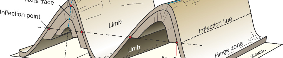
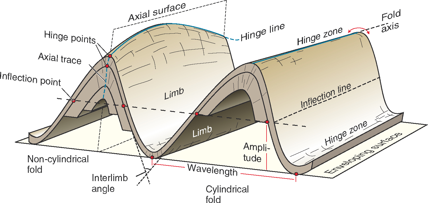
The folds are best observed perpendicular to their axial surface (Figure 1). In other words, you should be able to observe both limbs (Figure 4) of the fold with hinge points facing you. But we do not live in an ideal world. More often than not, only some parts of folds are visible. Using structural geology and engineering methods, we can still derive the necessary data from limited information. In fact, this is where a skilled Geoscientist or an Engineer can shine.

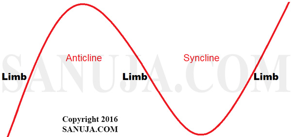
Anticline versus Syncline

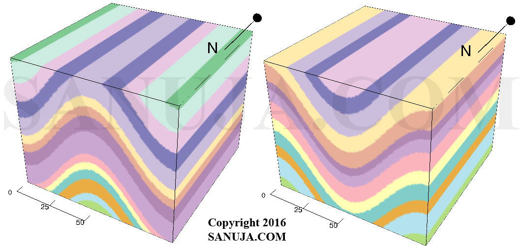
Cross-sections of folds can be used to interpret the geometry. Folds will form either concave down “hat-like” or concave up “cup-like” structures. The concave down structures (formations) with two limbs (explained under further down) pointing down are known as anticlines. You can remember this by associating the shape of letter A, which resembles the shape of an anticline. The concave up structures with two limbs pointing up are known as synclines. The following figure shows two 3D models of an anticline and a syncline.

Anticline versus Antiform and Syncline versus Synform

According to the Law of Superposition, the top (the highest) layer of sediment should be the youngest both on Anticlines and Synclines. However, if the oldest layer of an anticline is at the very top, we can classify it as an overturned anticline. We refer to such syncline as overturned syncline.

When the age information of the strata is not available or questionable, Geoscientists often refer to anticlinal shaped structures as antiforms. For opening upwards synclinal shaped structures, we call them synforms.

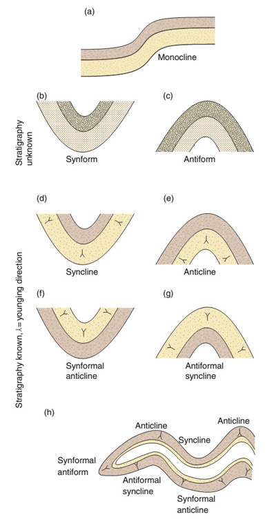
Additionally, when describing recumbent folds following terms are used. The term antiformal anticline is used for describing an antiformal fold with the oldest rocks in the core. The term, synfomal syncline is used when synclinal fold has the youngest unit in the core. The term, antiformal syncline is used for describing antiformal folds that have the youngest unit in the core while synformal anticline is used to describe synformal folds with oldest rock unit in the core.

Limbs and the Axial Plane

When describing a fold, the term “right limb” or “left limb” is used to refer to rock layers that have right and left sinusoidal curves. The following figure graphically illustrates the typical definition for a limb.

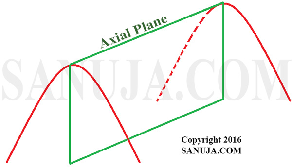
The axial plane or axial surface is at the very top or bottom in which the limbs are on either side of it. The axial plane can be defined as the plane or surface that divides the fold as symmetrically as possible. In other words, it is an imaginary line or surface of symmetry.

Hinge Line, Point and Zone

The hinge line, is defined as the imaginary line that connects points (touches the surface of) maximum curvature of a fold. For cylindrical folds, the hinge line and fold axis are the same.

The hinge zone is an imaginary plane, as opposed to a line, where maximum curvature of the fold occurs. A hinge plane is a surface of symmetry for cylindrical folds.

A hinge point is what you would observe on a cross sectional view of the hinge line on the surface of the fold.

Amplitude, Wavelength and Symmetry

Fold geometry can also be categorized by describing the folding pattern using amplitude, wavelength and symmetry. The amplitude can be measured if there is a visible complete anticline-syncline pair. Otherwise it could be a difficult task since each limb of a fold could extend further down into the subsurface making it difficult to identify the period. The amplitude of a periodic variable is a measure of its change over a single period. But we could use the inflection point on each limb to measure the amplitude. The inflection is the point on which the slope of the limb changes its direction. Figure 1 above is a diagram of anticline – syncline – anticline labeled with parts of folds.

Cylindricity

The classification cylindrical and non-cylindrical folds is based on the geometry of the hinge line or fold axis (Figure 1). Folds with straight hinge lines are known as cylindrical folds while the folds with curved hinge lines are known as non-cylindrical folds. The cylindricity varies depend on the stress experienced by the fold. In nature, non-cylindrical folds are very common. However, even cylindrical folds on large scales are often classified as non-cylindrical folds. This is expected since the cylindricity is actually a mathematical model rather than an observational one. It is very difficult to observe perfect symmetry in nature.

Also on Figure 1, the left anticline is non-cylindrical because the hinge line is curving. The right anticline is cylindrical because the hinge line is straight.

Cylindrical verses Conical

Cylindrical folds and conical folds have similar axial geometry. However, conical folds narrow the areas as they move along the hinge. In other words, conical folds reduce the structure to a point, just like a cone, when move along perpendicular to the maximum fold surface.

Cylindrical folds maintain (more or less in nature) the cylindrical shape as we move along the fold axis. When working in the field, d one should not get confused between conical folds and plunging cylindrical folds. Often Geologists make the mistake of classifying plunging cylindrical folds as conical folds.

Additionally, due to the variation in stresses and the variation in material strength, ductility, etc., folds can be observed in several different shapes such as kink, chevron, concentric and box (Figure 7).

Symmetry

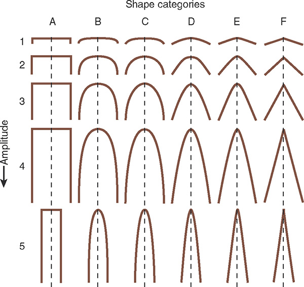
The geometric symmetry has been used by Hudleston (1973) to classify folds. It is based on the general shape of the fold. Others have developed several mathematical formulations to describe fold geometry. This is based on several variables such as amplitude, wavelength and period.

Orientation of Hinge Line and Axial Plane

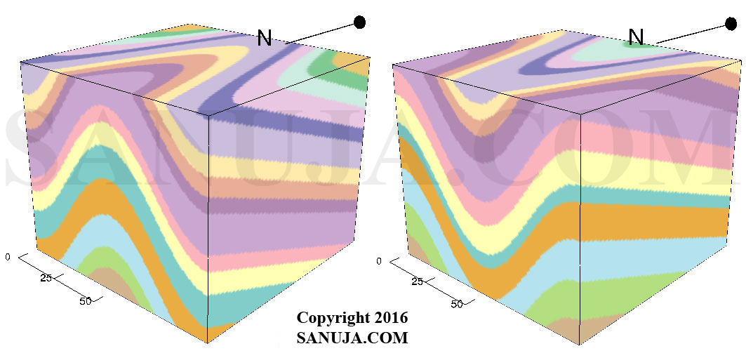
Plunging folds are folded structures that have a “dip” along the hinge line. The term “plunging fold” is used to describe what happens when the entire fold is plunging up or down. It should not be used to describe change in orientation of a single layer of the fold. The axial surface along with the hinge line changes orientation in plunging folds. The following figure shows two 3D models of a plunging anticline and a plunging syncline. Notice the beds plunging steeply into the subsurface.

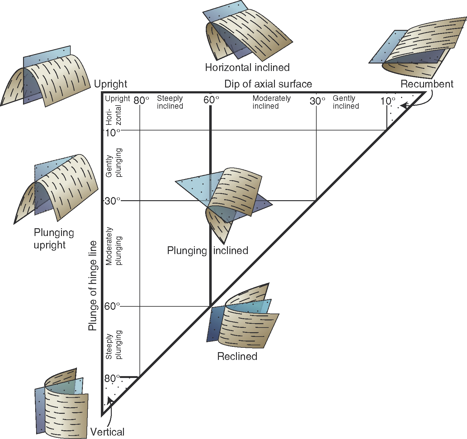
Fleuty (1964) has classified the folds based on this concept as Upright, Plunging; Upright, Vertical; Reclined; Plunging Inclined; Horizontal Inclined and Recumbent (Figure 9) based on the orientation of the hinge line.

The Hudleston (1973) classification relies on the shape and the amplitude categorization (Figure 10).

These are just two examples because there are several different classifications in use today. But the primary objective is to classify based on the geometry and the orientation of the folds. While ones view of folds may vary from geologist to geologist, field observations should always be recorded as to what was observed and measured in the field. Depending on whom you talk to, these classifications may be modified. One of the few universal methods employed by geologists is to measure the distance between the two limbs on a stereonet. This will provide the information needed to determine the tightness of the fold.

Dip Isogons

Dip isogons are imaginary lines that can be drawn between two points of equal dip within the fold structure. They are straight lines that can be used to connect inner and outer boundaries of folded layers. The orientation of dip isogons can be used to classify folds into three classes. Imaginary lines between fold plains are used for analysis of geometry.

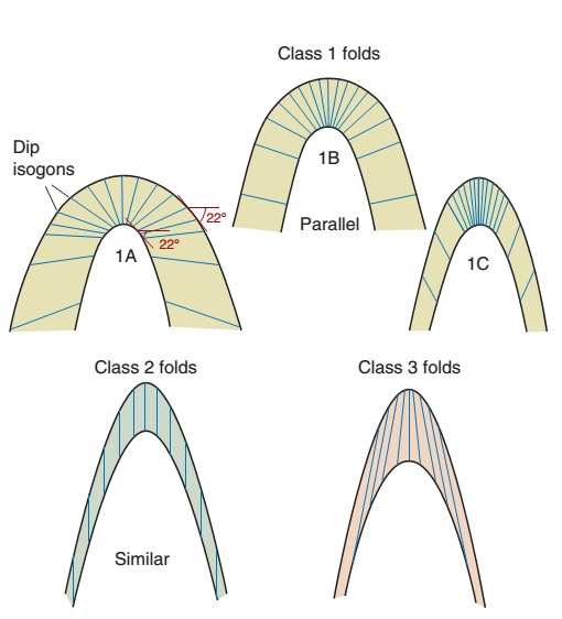
Class 1 – The dip isogons converge toward the inner arc, which is tighter than the outer arc.

Class 1A – The dip isogons have the same characteristics as the Class 1, but the limbs have a larger thickness (thicker) than the hinge.

Class 1B – The dip isogons have the same characteristics as the Class 1, but the thickness remain consistent (same) hence it is a parallel fold.

Class 1C – The dip isogons have the same characteristics as the Class 1, but the limbs have smaller thicknesses (thinner) than the hinge.

Class 2 – The dip isogons are parallel hence the inner and outer arc curvatures are the same. It is known as a “similar fold”.

Class 3 – Is characterized by parallel dip isogons with no convergence on either side. The Class 3 type has the isogons converging toward the outer arc.

The most common classes of folds are Class 1B and Class 2 folds. However, depending on the area of interest (eg. Canadian Rockies) and variations in respective layer properties, one class of folds may be more common than another.

Cleavage

Cleavages are usually formed parallel to the axial surface; axial plane cleavages. They will continue to orientate along the direction of the slip while fold is being formed. Depending on the type of material in each layer and the variation of viscosity between them can cause cleavage orientation to change. This is known as cleavage refraction, which is also influenced by pre-folding, layer-parallel shortening and flexural shear during folding.

The growth of cleavages are directly related to the principle stress axis (always elongate in the direction of least force), thus we can use them to identify the XY-plane of the strain ellipsoid.

Folds and Folds

The smaller folds (active folds) or buckling can be used to determine the deformation history. When a fold is formed in a region where there has been a compressional event earlier, this can be used to identify the limbs and the axial trace. The Z-folds on an anticline will indicate the left limb, the S-folds will indicate the right limb and the hinge zone will have the M-folds. Z, M and S folds.

Flexure Geometry

During folding events, if the strain is more evenly distributed in the limbs in the form of shear strain, as is more common in a plastic regime, flexural slip turns into flexural flow or shear. Orthogonal flexure produces parallel folds with a neutral surface while pure flexural folds folds with no neutral surface, and strain increased away from the hinge line.

Orthogonal flexure is classified as Class 1B because all the lines originally orthogonal to the layering will maintain their orientation during the entire deformation history.

Flexural slip on the other hand indicates slip along layer surfaces or very thin layers during folding. Slickenlines (slickensides) on foliated layers and constant bed thickness reveal flexural slip.

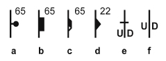
Folds on a Map

Historically, there have been several different symbols used by geologists to denote folds on maps. As of 2003, we do not have an international standard set of symbols. Hence, we have to rely on information from the publisher, year of publication, the place of publication and other appendices of the map to obtain data. Most maps include a legend with all the symbols clearly described. These are usually printed either on a side or back of the map. Conventionally all geologic maps should be printed with North pointing up; but be sure to confirm this on your map before you extract data. Some of the common symbols we use for folds today are shown in Figure 16 and 17.

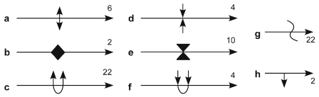
For more information on map reading, please read How to read Geological Maps.

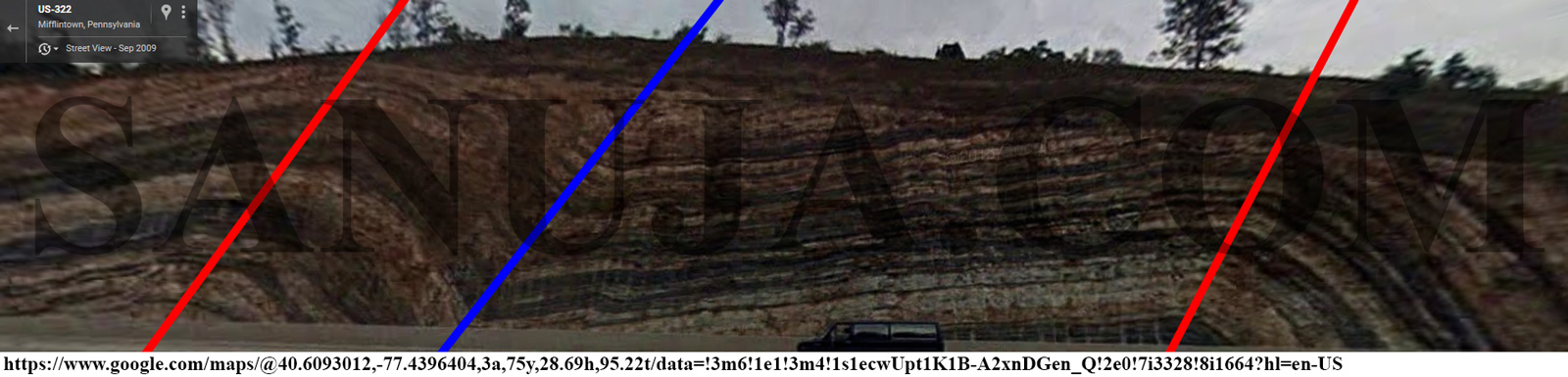
Real world example

With programs like Google Maps and Google Earth, you can study folds without leaving your room. Here is an example of lazy method where Google Street View of a syncline bounded by two anticlines on either sides.

References

1) Images Credit: Structural Geology by Haakon Fossen

2) Images Credit: 3D Structural Geology; A Piratical Guide to Quantitative Surface and Subsurface Map Interpretation SE; Groshong, Jr., 2006

3) Images Credit: Google Street View original – Click Here

4) Images Credit: VisibleGeology Beta by Rowan Cockett

Further reading: 341 Final Exam Materials

Edited by: Nicholas Coffey, Chief Scientist, Coffey Geoscience, Salem OR
Updated: 16-Aug-2016