Introduction
Interference figures or some text may refer to as optical figures are used by mineralogists and other scientists to describe optical properties of crystals. In Geology, optical properties of naturally occurring crystals are used to identify and classify minerals. In addition some companies are interested in manufacturing economically valuable minerals such as synthetic diamonds have a growing interest on the behaviors of these figures.
The interference figures are produced when the polarized light is “split” by a crystal as a result of its physical and chemical properties. However, most textbook will refer to these properties as optical properties. Remember optical properties are caused by physical and chemical variations within the mineral. To obtain an interference figure, the mineral must be anisotropic (as opposed to isotropic).
A petrographic microscope (polarizing transmitting light microscope) must be setup the following way to obtain an interference figure:
1) Focus on a grain under Medium power objective lens on the center of the cross hair.
2) Switch the objective lens to High power (40X and up).
3) Flip the Condenser lens to the path of the light ray.
4) Insert/flip the Polarize to the path of the light that traveled through the mineral.
5) Insert the Bertrand lens and focus it (or remove the ocular lens).
6) Use the Accessory plate to determine the sign (+/-) of the figure. The measurements of vibration is always depend on the slow direction of the Accessory plate.
Uniaxial Minerals
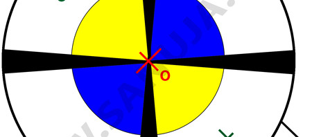
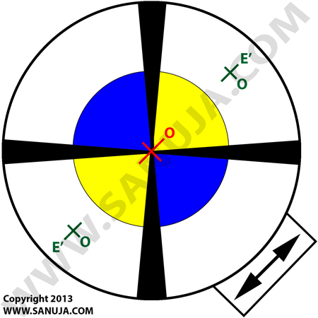
The light will be slip into two components; epsilon (ε) and omega (ω). Following is an example of such image obtained using a microscope. Only one Optic Axis hence, the angle of which the isogyres (bands of extinction – black lines) form is 90-degrees.
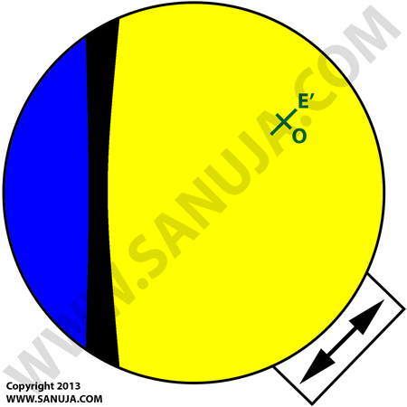
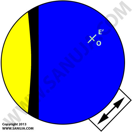
The following is the same crystal when the Accessory Plate is inserted. Since the upper right has a blue isochrome (colour curves), it is clearly a positive mineral. But take a note that while the diagrams in textbooks may indicate strong blue and yellow regions with clear separations between them, it is just a representation of the following image.
Uniaxial Negative Figures
The value of component ε less than the value of component ω. Hence, will produce a negative interference figure.
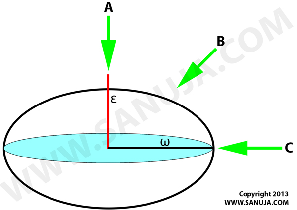
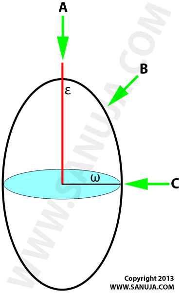
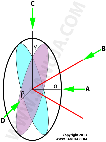
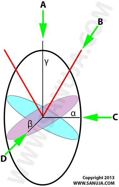
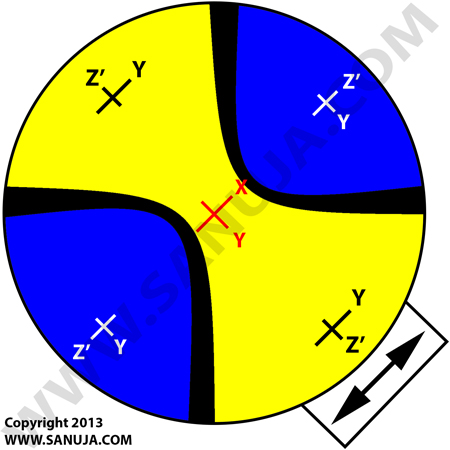
Scenario A – If you are looking down at the Optic Axis (A on Figure 1 – above), in which the mineral is cut perpendicular to the Optic Axis, then a Centered Optic Axis interference figure (Figure 2 – below) can be obtained. In uniaxial we can only measure the O – vibration direction.
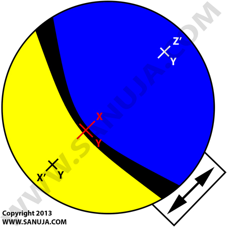
Scenario B – This is a situation where you are looking down the crystal in between the two vibration directions, but further away from the omega (ω). With each rotation of the stage, the interference figure will move around the field of view.
Scenario C – When a mineral is cut parallel to the optic axis, you will be looking down at C axis. This will produce a Flash figure. It is not very useful for Interference Figure analysis, but this type of figure is best used for determining birefringence.
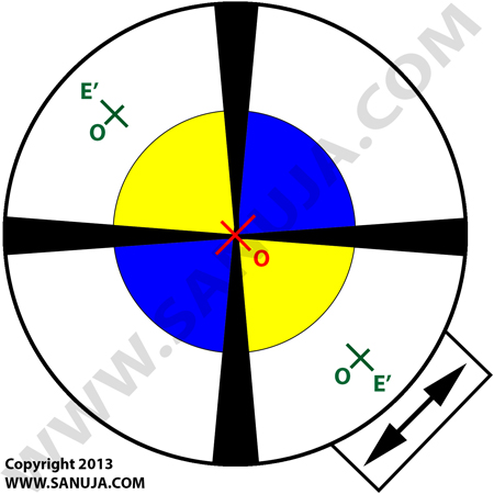
Uniaxial Positive Figures
The value of component ε greater than the value of component ω. Hence, will produce a positive interference figure.
Scenario A – Bxa interference figure
Scenario B – Optic Axis interference figure
Biaxial Minerals
Biaxial Negative Figures
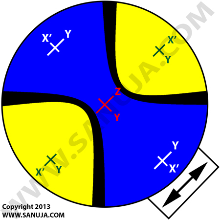
Scenario A – Between the 2-Optic Axises. Figure 8 below. This is a special Interference Figure known as Acute Bisectrix Figure (Bxa).
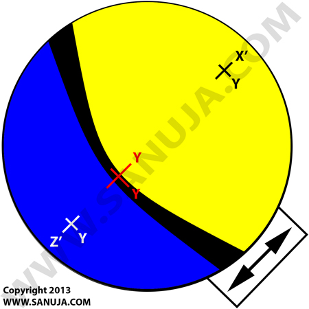
Scenario B – Optic Axis based interference figure.
Scenario D – This will results in a Flash figure. Useful for determining birefringence, but not helpful in obtaining an interference figure.
Biaxial Positive Figures
Scenario A – Between the 2-Optic Axises. Figure X below. This is a special Interference Figure known as Acute Bisectrix Figure (Bxa).
Scenario B – Optic Axis interference figure.
Scenario D – This will results in a Flash figure. Useful for determining birefringence, but not helpful in obtaining an interference figure.