Data Collected From the Map

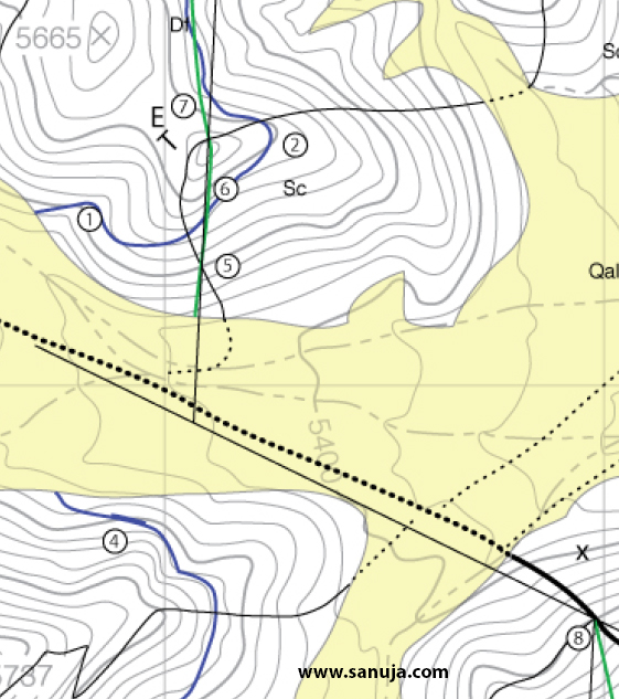
Only one strike lines is drawn on the Figure 1 for the fault, but it is recommended to draw at least two of them to measure the dip of each feature. The line that go across point 5 (Figure 1) is the piercing (“pin line”) obtained from the steronet (Figure 3).

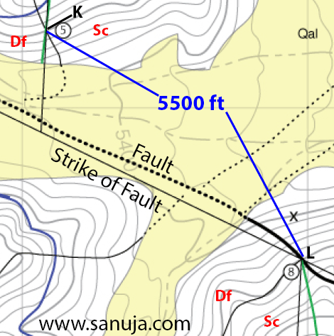
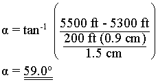
The dip of the fault is calculated using its strike lines 5500 ft and 5300 ft. It was calculated:

The strike is measured on the map as 269-degrees. The intersection between the bedding planes is defined as the piercing point.

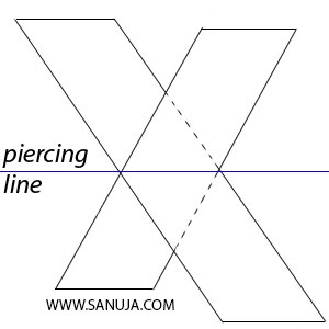
The intersection between two plains result in a line of contact along the axis. This line is known as the piercing line.

Plot on the Stereonet

When plotting on stereonets, make sure you take the apparent dip and not the true dip.

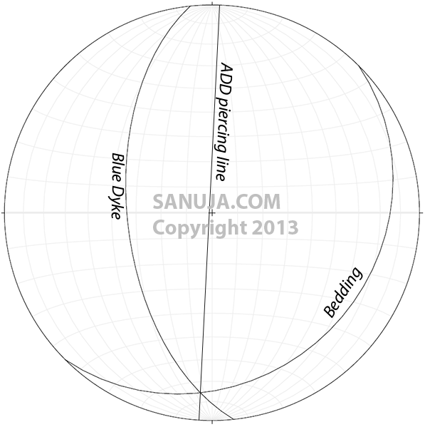
The intersection point on the Figure 4 is used for determining the trend and plunge of the piercing line. It was 183/21 degrees. Now you can plot this on the map itself as it has been already done in Figure 1.

3D Fault Block

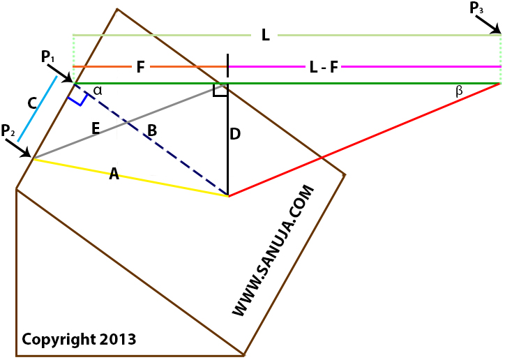
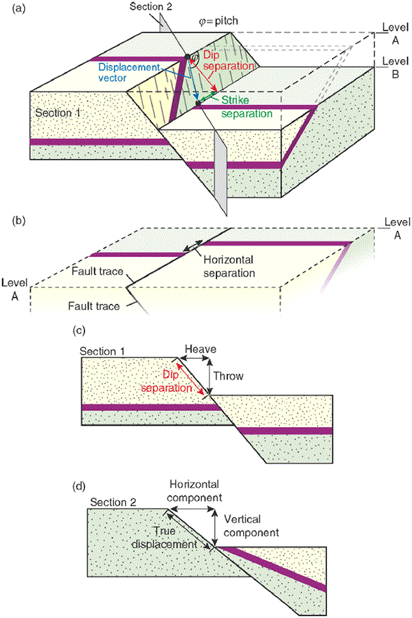
On the Figure 5 3D block diagram;
angle α = dip of the fault
angle β = dip of the piercing line (stereonet; the trend and plunge)
A = net-slip: total slip of the fault
B = dip-slip (dip shit? no): dip of of the parallel component to the slip
C = strike-slip component; parallel slip component
D = vertical throw; vertical component of the net-slip
E = horizontal throw; horizontal component of the net-slip
F = heave; the stratigraphic apparent horizontal component of the net-slip

Identification letters on the block is chosen as a compliment to this diagram (click here).

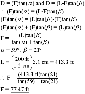
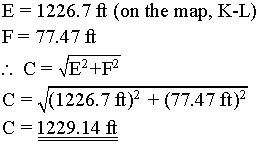
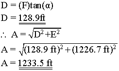
Therefore, we get 77.47 ft for the heave (UofC answer key has 79 ft due to map errors and such) and it will translate into about 0.58 cm on the map. Using this information we can now calculate the horizontal throw.

The vertical throw and the net-slip (slip vector) can be found using;

Here is a 3D visualization of a faulting event.